Mastering Binary Classification with Pure TensorFlow: An In-Depth Step-by-Step Guide

In this blog post, we will dive into the world of binary classification using TensorFlow, covering essential concepts like variables, operations, gradients, and more. Binary classification is a fundamental task in machine learning, where the objective is to categorize data into one of two distinct classes. By generating synthetic data, building a logistic regression model, and training it with TensorFlow, you'll gain hands-on experience and a deeper understanding of this crucial machine learning technique.

Generating Synthetic Data

First, we need some data to start working with. We will generate synthetic data using the numpy.random.multivariate_normal function. This function computes coordinates from a random distribution with a predefined covariance matrix and mean. The covariance matrix describes the shape of the point cloud, while the mean indicates its position in the plane. To create two classes, we will use the same covariance but different means.

# First import necessary libraries
import tensorflow as tf
import numpy as np
import matplotlib.pyplot as plt

# Generate synthetic data
num_samples = 2000
class_0_samples = np.random.multivariate_normal(
    mean=[0, 4], cov=[[1, 0.4], [0.4, 1]], size=num_samples
)
class_1_samples = np.random.multivariate_normal(
    mean=[4, 0], cov=[[1, 0.4], [0.4, 1]], size=num_samples
)
features = np.vstack((class_0_samples, class_1_samples)).astype(np.float32)
labels = np.vstack((
    np.zeros((num_samples, 1), dtype=np.float32),
    np.ones((num_samples, 1), dtype=np.float32)
))

Visualizing Data for Better Insights

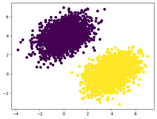
Visualizing the dataset helps us understand the distribution and separation of the two classes.

# Visualize the dataset
plt.scatter(features[:, 0], features[:, 1], c=labels[:, 0])
plt.show()

Here is what our dataset looks like:

Formulating the Logistic Regression Model

The core of our binary classification model is represented by the logistic regression formula:

$$\begin{equation} y = \sigma(w^\top x + b) \end{equation}$$

where σ is the sigmoid function, w are the weights, b is the bias term, and x is the input vector.

Initializing Model Parameters with TensorFlow

We initialize the model's parameters using TensorFlow variables. Weights are initialized with tf.random.uniform to ensure randomness and prevent symmetry, while biases are set to zero using tf.zeros.

input_dim = 2
output_dim = 1
weights = tf.Variable(tf.random.uniform((input_dim, output_dim)))
bias = tf.Variable(tf.zeros((output_dim,)))

Defining the Logistic Regression Model in TensorFlow

We define the logistic regression model using TensorFlow operations.

def logistic_model(inputs, train=False):
    z = tf.add(tf.matmul(inputs, weights), bias)
    if train:
        return z
    return tf.sigmoid(z)

Implementing the Binary Cross-Entropy Loss Function

The loss function used for binary classification is binary cross-entropy loss.

$$\begin{equation} \text{Binary Cross-Entropy Loss} = -\frac{1}{N}\sum_{i=1}^{N} \left[y_i \log(\hat{y}_i) + (1 - y_i) \log(1 - \hat{y}_i)\right] \end{equation}$$

In TensorFlow, we implement it as follows:

def binary_crossentropy_loss(true_values, predicted_values):
    return tf.reduce_mean(
        tf.nn.sigmoid_cross_entropy_with_logits(labels=true_values, logits=predicted_values)
    )

Implementing the Training Step/ Backpropagation

The training step involves calculating the loss, computing gradients, and updating the model parameters.

learning_rate = 0.1
def train_step(features, labels):
    with tf.GradientTape() as tape:
        logits = logistic_model(features, train=True)
        loss = binary_crossentropy_loss(labels, logits)
    gradients = tape.gradient(loss, [weights, bias])
    weights.assign_sub(gradients[0] * learning_rate)
    bias.assign_sub(gradients[1] * learning_rate)
    return loss

Accuracy Metric

The accuracy metric calculates the proportion of correct predictions by comparing the predicted classes to their true values.

def accuracy(true_values, predicted_values):
    predicted_classes = tf.cast(predicted_values > 0.5, tf.float32)
    correct_predictions = tf.cast(tf.equal(predicted_classes, true_values), tf.float32)
    return tf.reduce_mean(correct_predictions)

Training the Model

We train the model for 10 rounds, printing the loss and accuracy at each step.

num_steps = 10
for step in range(num_steps):
    loss_value = train_step(features, labels)
    predictions = logistic_model(features)
    acc_value = accuracy(labels, predictions)
    print(f"Loss at step {step}: {loss_value:.4f}, Accuracy: {acc_value:.4f}")

After 10 rounds, the loss is 0.1533, and the accuracy is 0.9995, which is quite impressive.

You can find the code at the GitHub repository.

Note: The code is a modified version for classification of deep learning with the Python book github repository for educational purposes.